π₀, explained: turning a vision-language model into a robot with flow matching

01Why start from a vision-language model

The hard part of a general-purpose robot is not the motors, it is the understanding. To bus a table, the robot has to know that a crumpled napkin is trash and a fork is not, that "put the dishes away" implies an order of operations, that a half-seen mug behind a glass is still a mug. None of that lives in a robot dataset. It lives on the internet, in the captioned images and text that vision-language models (VLMs) are already trained on.

So the move is to not start from scratch. Take a VLM that has digested internet-scale image and text data, and graft a body onto it. Keep the semantic understanding, add the ability to emit motor commands. The result is a Vision-Language-Action (VLA) model: same transformer that reads pixels and language, now also speaking in actions.

◆ analogy

It is the difference between teaching a toddler to fold laundry and teaching a literate adult who has read about laundry, seen a thousand photos of folded shirts, and just needs to learn the motor skill. The adult does not need to relearn what a shirt is. π₀ wants the robot to arrive at the task already knowing the world, so the only thing left to learn from robot data is how to move.

02The anatomy of π₀: one transformer, two specialists

π₀ is one transformer with two sets of weights. The first set is the pretrained VLM backbone, PaliGemma, an open-source 3-billion-parameter VLM (a SigLIP-So400m vision encoder plus a Gemma 2B language model). The second set is a newly initialized action expert, roughly 300M parameters, that handles the robotics-specific inputs and outputs (the robot's joint state and the action tokens). Together they total about 3.3 billion parameters.

The design is borrowed from Transfusion: a single transformer trained with different objectives on different tokens. Image and language tokens are supervised the way a VLM is supervised; action tokens are supervised with a flow-matching loss (section 5). Because the two kinds of tokens are routed through two weight sets but share one attention stack, π₀ behaves like a small mixture of experts with exactly two elements: a VLM expert for perception and language, an action expert for state and motion. They are separate parameter banks, but they talk to each other on every layer through self-attention.

▲ why a separate expert at all

You could feed actions through the same weights as text. The authors found that giving the robotics tokens their own weights improved performance. The intuition: predicting a continuous motor command is a genuinely different computation from predicting the next word, so let it have its own parameters, while still letting it read everything the VLM understood about the scene.

Two camera views from a LeRobot dataset frame: a phone-mounted view and a laptop view of a tabletop arm — **Figure 2.** One frame of robot data, the way π₀ consumes it. Multiple camera views, a language instruction ("grasp a lego block and put it in the bin"), and the robot's current joint angles. Those three things together are the observation the model conditions on. (Frames shown from a LeRobot SO-100 recording, a stand-in for the same observation structure; π₀'s own data uses 2 to 3 robot cameras, not these phone and laptop views.)

03Action chunking: predict a whole burst of motion at once

A robot controlled at high frequency takes many small steps per second. If the model predicted only the next action each time, the stream would tend to stutter and the inference cost would dominate. π₀ instead predicts an action chunk: a block of H = 50 future actions in a single forward pass. The robot then executes that burst, which is what lets it run smoothly at up to 50 Hz on dexterous tasks.

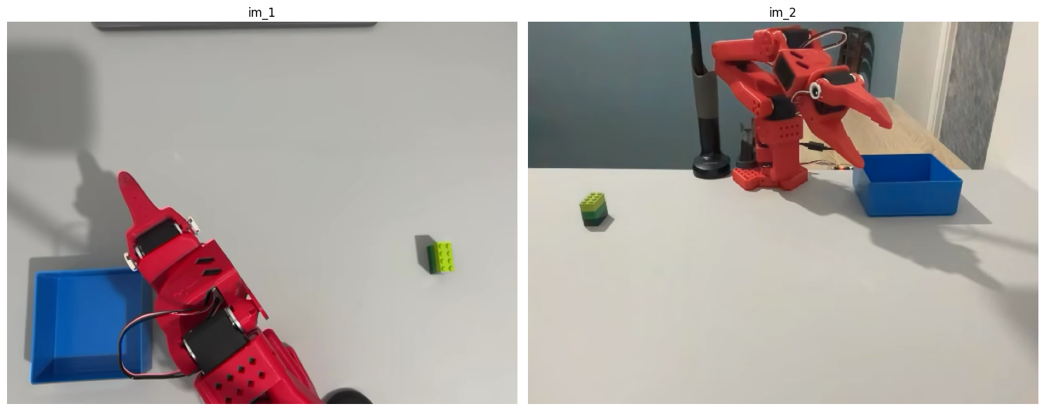
What does the model condition on to produce that chunk? An observation $o_t$ assembled from exactly the three ingredients in Figure 2:

$$o_t = \big[\, I_t^{1},\, \dots,\, I_t^{n},\; \ell_t,\; q_t \,\big] \;\longrightarrow\; A_t = [\,a_t,\, a_{t+1},\, \dots,\, a_{t+H-1}\,],\quad H=50$$

In words: $I_t^{i}$ are the camera images (2 to 3 views per robot, missing slots masked out), $\ell_t$ is the language instruction tokenized, and $q_t$ is the robot's current joint configuration. From that, π₀ predicts $A_t$, the next 50 actions, as one object. It is modeling a distribution $p(A_t \mid o_t)$ over whole chunks, not a single mean step.

In code, with the LeRobot data format, an observation is nothing more exotic than stacking the frame's fields:

▮ one observation, in code

frame = data[0] → O_t = [ frame['observation.images.phone'], frame['observation.images.laptop'], frame['task'], frame['observation.state'] ]. The 'task' string is the language command, 'observation.state' is the joint-angle vector $q_t$, and the label the model must learn to produce is frame['action'], a chunk of future motor targets. That is the entire interface.

04Why not just regress the actions?

Here is the temptation: actions are vectors of numbers, so just train the network to output them directly with a mean-squared-error regression. For many control problems that works. For dexterous manipulation it quietly fails, and the reason is multimodality.

Often there is more than one correct way to act. To grasp a block you can come in from the left or from the right; both are valid, expert demonstrations. Now ask a regressor, trained to minimize squared error, what to do. It cannot output "left or right." The single output that minimizes its loss against a mix of left and right demos is the average of the two: come in straight down the middle, exactly where the block is, exactly where nothing can grasp it. The mean of two good actions is often a bad action.

Flow matching dodges this. Instead of predicting one point, it learns a field that pushes a random starting point toward a valid action, and crucially the field lets samples commit to one mode. Some random seeds flow to the left grasp, others to the right, none get stuck averaging in the dead center. Drive it yourself below: toggle between a plain regressor and flow matching, and set how many integration steps the flow gets.

★ the key insight

Regression collapses a multimodal action distribution to its mean, and the mean of valid actions is frequently invalid (a grasp of nothing, a path through an obstacle). Flow matching represents the whole distribution and produces samples that each pick a mode, so the chunk you get out is a real action, not an average of incompatible ones. This is exactly the property dexterous, high-frequency control needs.

05Flow matching, made concrete

The mechanism is simpler than the name. Pick a straight line between pure noise and a real action chunk, and teach the network the velocity along that line. At inference you start at noise and follow the velocity to the real action.

1. The noisy interpolation

Take a real action chunk $A_t$ from the data and draw Gaussian noise $\epsilon \sim \mathcal N(0,I)$. Define a noised version that slides linearly from noise (at $\tau=0$) to the clean chunk (at $\tau=1$):

$$A_t^{\tau} = \tau A_t + (1-\tau)\,\epsilon,\qquad \tau\in[0,1]$$

In words: this is the conditional probability path $q(A_t^{\tau}\mid A_t)=\mathcal N(\tau A_t,\,(1-\tau)I)$, a straight line in action space; the blend is mostly noise near $\tau=0$ and mostly the real action near $\tau=1$.

2. The target the network learns

Differentiate that line and you get its constant velocity, the direction that carries a noisy point toward the clean one. That is the target vector field:

$$u(A_t^{\tau}\mid A_t) = A_t - \epsilon$$

In words: "from this noisy point, the ideal direction to move is $A_t - \epsilon$." The network's job is to predict that direction from the noisy input, the timestep, and the observation, even though at test time it never sees the true $A_t$ or $\epsilon$.

3. The loss

The action expert outputs a predicted field $v_\theta(A_t^{\tau}, o_t)$, and training is just mean-squared error between the prediction and the target. That is the whole flow-matching objective:

$$L^{\tau}(\theta) = \mathbb E_{\,p(A_t\mid o_t),\,q(A_t^{\tau}\mid A_t)} \;\big\lVert\, v_\theta(A_t^{\tau}, o_t) - u(A_t^{\tau}\mid A_t)\,\big\rVert^2$$

In words: sample a real chunk and an observation, corrupt the chunk to noise level $\tau$, ask the network for the velocity, and penalize how far it is from the true velocity $A_t - \epsilon$. No special losses, no adversarial games. It is regression, but on the field rather than on the action.

◆ analogy

Think of every noisy point as a hiker dropped somewhere in fog, and $v_\theta$ as a compass the model is learning to build. Training shows the compass thousands of (position, correct-bearing) pairs. At test time the hiker has no map, only the compass, and walks one short step at a time. Because different starting points get bearings toward different valid summits, two hikers near the dead center can peel off toward different grasps instead of both freezing in the middle.

06Inference is iterative denoising

Generating an action chunk is the reverse of corrupting one. Start at $\tau=0$ with a fresh draw of pure noise $A_t^{0}\sim\mathcal N(0,I)$, then repeatedly step along the learned field with forward Euler until you reach $\tau=1$:

$$A_t^{\tau+\delta} = A_t^{\tau} + \delta\, v_\theta(A_t^{\tau}, o_t),\qquad \delta = 0.1$$

In words: ask the network which way to move, take a small step that way, advance the clock by $\delta$, repeat. π₀ uses 10 integration steps ($\delta=0.1$), so ten forward passes turn a cloud of noise into a clean 50-step action chunk.

This is the same loop the widget in section 4 was running. Each Euler step is one short move along the polyline you saw; with very few steps the path is coarse, with around ten it lands cleanly on a mode. Drag the integration-steps slider on the grasp widget in section 4 back up and watch the path tighten onto a real grasp. Ten is the sweet spot π₀ uses: enough to be accurate, few enough to stay real-time.

▲ a convention to keep straight

In this paper $\tau=0$ is noise and $\tau=1$ is data, so inference integrates from 0 up to 1. (Some flow-matching papers flip the direction; here, low $\tau$ means high noise.) That orientation matters for the next section, because it decides which timesteps are the hard ones.

07The detail that matters: oversample the hard, high-noise steps

During training you have to pick a $\tau$ for each example. The lazy choice is uniform. But the authors reasoned that the hardest part of denoising is the very beginning, near $\tau\approx 0$, where the input is almost pure noise and the model has to commit to a direction with almost no signal to go on. So they sample $\tau$ from a Beta-shaped schedule that oversamples the high-noise (low $\tau$) regime, spending more of the training budget where the model needs the most help. (They also cap the sampled $\tau$ just below 1, since the easiest, almost-clean steps need little practice.)

Drag the schedule's shape below to pile more or less training mass into the hard, high-noise region. The shaded band is the part of the process where the model is working with the least information; watch how much of its training time lands there.

Test yourself: why does sampling τ near 0 more often make the model better?

Near $\tau=0$ the input is almost pure noise, so the correct velocity is the hardest to infer: there is barely any signal pointing toward a valid action, and getting the direction wrong this early sends the whole Euler trajectory toward the wrong mode (or the dead average). Near $\tau=1$ the input is already almost the real action, so the remaining correction is tiny and easy. By oversampling low $\tau$, the model spends most of its capacity practicing the step where mistakes are most expensive and least forgiving, which is exactly the step that decides which mode a sample commits to. Drag the shape slider above: pushing mass toward $\tau\to 0$ is the schedule doing precisely that.

08How information flows: the attention mask and the cache trick

One transformer, two experts, but who is allowed to look at whom? π₀ groups its tokens into three blocks and uses a deliberately block-wise causal attention mask to control the flow:

Block ①, images + language: attends only within itself. It cannot peek at the robot state or the actions. This protects the VLM's pretrained understanding from being warped by robotics-specific inputs it never saw on the internet.
Block ②, robot state $q_t$: attends to ① and to itself, but not to the actions. Because the state is fixed during a chunk's generation, its keys and values can be computed once.
Block ③, noisy actions $A_t^{\tau}$: attends to everything, ①, ②, and bidirectionally to itself. The whole chunk is denoised jointly, conditioned on the full context.

Click a query block below to see exactly which keys it is allowed to read under π₀'s mask, then flip to a fully bidirectional mask to see what the design deliberately gives up.

★ the cache trick that makes it real-time

Look at what the mask buys you at inference. Blocks ① and ② never attend to the actions, so their keys and values do not change across the 10 denoising steps. Compute the image, language, and state prefix once, cache its keys and values, and every Euler step only has to recompute the small action block (③) against that frozen cache. Ten denoising steps, but the expensive 3-billion-parameter VLM prefix runs a single time. That is how a 3.3B model controls a robot at 50 Hz.

09The training recipe: broad and crude, then narrow and clean

Architecture is half the story; the other half is data, and π₀ borrows the LLM playbook: a huge, diverse pre-training phase followed by smaller, high-quality post-training.

10,000+ h

robot data in pre-training, plus the Open X-Embodiment mixture (22 robots)

7 · 68

robot configurations and tasks in Physical Intelligence's own dataset

~3.3B

total parameters: PaliGemma backbone (~3B) + action expert (~300M)

H=50 · 50 Hz

action chunk length and control rate on dexterous tasks

Pre-training is deliberately broad and a little crude. It mixes single-arm, dual-arm, and mobile manipulators, with the entire OXE corpus on top. Diverse but inconsistent data is a feature here: it teaches the model the full range of physical interaction and how to recover from mistakes, because mistakes (and their corrections) actually appear in messy data. To stop the data-rich tasks (laundry folding has a lot of footage) from drowning out the rest, each task-robot combination is down-weighted by roughly $n^{0.43}$, where $n$ is its sample count.

Post-training then fine-tunes that generalist on a small, clean, task-specific dataset to make it fluent and reliable at one job. How much data depends on the task: the simplest adaptations need around 5 hours, the hardest (mobile laundry folding) use 100 or more hours of high-quality demonstrations.

● the honest hype check

Read that last number again. Even after more than 10,000 hours of pre-training, each genuinely new, complex task still needs tens to a hundred-plus hours of fresh, high-quality demonstrations. π₀ is a real advance in how much a single model can absorb and how fluently it moves, but it does not make robot data cheap, and it does not make general-purpose embodied intelligence imminent. The right framing is the LLM one: a strong base model that is far easier to specialize, not a finished generalist. Progress is real; the hype outruns it.

10Where it fits, and where it breaks

π₀ is the cleanest early statement of a now-standard idea: a VLA is a pretrained VLM with an action generator grafted on. The two design choices that make it work are worth carrying forward. First, generate actions by flow matching rather than regression, so the model can represent multiple valid motions and commit to one instead of averaging them into a collision. Second, use a block-wise mask plus a cached prefix so a multi-billion-parameter model can still emit action chunks fast enough for real-time, high-frequency control.

● honest limitations

The generalist base is impressive but not autonomous: complex tasks still demand substantial per-task fine-tuning data. Flow matching needs several integration steps per chunk (ten here), so the cache trick is load-bearing, not optional. And like any imitation-trained model, π₀ inherits the coverage of its demonstrations: behaviors and recoveries it never saw in data remain out of reach. It is a foundation to build on, not a solved problem.

The one-sentence takeaway: take a model that already understands the world from the internet, bolt on a small expert that turns noise into motion by following a learned velocity field, cache the expensive half so it runs in real time, and a vision-language model becomes a robot that can fold laundry.