Ambient Diffusion Policy, explained: learning good robot behavior from imperfect demonstrations

01The data-quality dilemma in robot learning

Every large robot policy is trained on a heterogeneous soup of data: a little expensive expert teleoperation, plus an ocean of cheaper, lower-quality stuff, failed attempts, simulation, cross-embodiment demonstrations, ego-centric human video. High-quality, task-specific data is slow and costly to collect; suboptimal data is abundant and only getting more so. Learning well from imperfect demonstrations is therefore not a temporary artifact of data scarcity, it is a permanent feature of how robot foundation models are built.

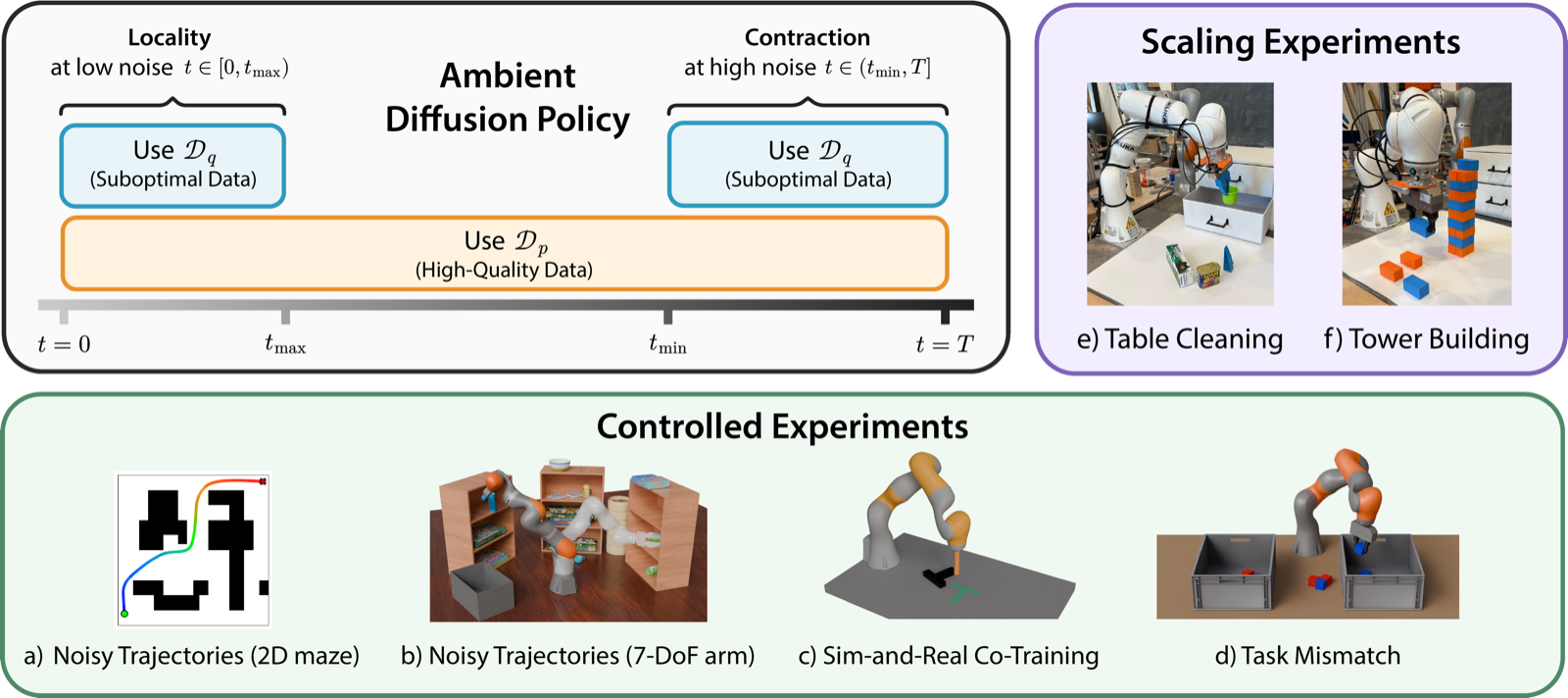
The goal is precise: given a small high-quality target set $\mathcal{D}_p$ (drawn from a distribution $p$) and a much larger suboptimal set $\mathcal{D}_q$ (from a shifted distribution $q$), train a policy that is good on the target distribution while still squeezing useful signal out of $\mathcal{D}_q$. The kinds of suboptimality studied are concrete: jittery trajectories, a sim-to-real gap, wrong high-level task logic, and large unstructured mixtures like Open X-Embodiment.

Two dominant recipes both fall short. Data filtering simply throws the low-quality samples away (Dexora drops 80% of its data; OpenVLA keeps only 27 of OXE's datasets). That is wasteful: even a bad demonstration usually carries some transferable signal. Co-training blends the two losses with one weight, $\alpha\,\mathcal{L}_{\mathcal{D}_p} + (1-\alpha)\,\mathcal{L}_{\mathcal{D}_q}$. But sampling from a mixture that contains $q$ fundamentally biases the policy toward $q$, teaching it both the meaningful and the harmful parts, and the weight $\alpha$ is a fragile knob you have to sweep.

★ the reframe

The field has long asked which data sources to include and how to weight them. Ambient Diffusion Policy asks a different question: when, at which diffusion noise level, should each source be allowed to teach? A single suboptimal demonstration can be wrong about the fine motion but right about the plan (or vice versa), so it should contribute at some noise levels and be excluded at others. That is impossible to express with one mixing weight.

02A hidden structure: robot actions are power-law

The key that unlocks everything is an empirical property of robot action data. Take any action signal over time, compute its power spectral density (how much energy sits at each frequency), and plot it on log-log axes. Across Open X-Embodiment (2.4M episodes, 70+ datasets) and six other robot datasets, the spectrum is a straight line: it decays as $|f|^{-\alpha}$, a spectral power law. Almost all the energy lives at low frequencies (slow, smooth, large motions), and fine jitter at high frequency carries very little.

$$S_X(f) = C\,|f|^{-\alpha}, \qquad \text{for } |f|\ge f_0,\quad C>0,\ \alpha>1,\ f_0\ge 1$$

In words: the empirical, distinguishing property of robot action data. The fitted exponent $\alpha$ sits comfortably above 1 across every robot dataset the authors measured (Figure 3a). Crucially this is not universal: natural audio, stellar spectra, and Poisson point processes do not have it, which is exactly what makes it a useful fingerprint of robot motion. Everything downstream, the hierarchy, the contraction, the locality, follows from this one fact.

Why does a power-law spectrum matter for a Diffusion Policy? Because diffusion is, in Dieleman's phrase, "spectral autoregression": a denoiser trained on power-law data generates low-frequency content at high noise and high-frequency content at low noise. Equivalently, adding flat-spectrum Gaussian noise to a power-law signal destroys the low-energy high-frequency components first. Noise behaves like a high-frequency mask that erases the fine local detail before it touches the coarse global structure.

◆ low-pass blur

Adding diffusion noise to a robot action is like progressively blurring a photo. The fine texture (jitter, a clumsy local wiggle) disappears first; the coarse shape (the route through the room) survives the longest. Two photos that differ only in fine texture become identical once you blur them enough. That is the whole intuition for why suboptimal data can be safe at high noise.

03Noise as a dial: the global-to-local hierarchy

Put those two facts together and the diffusion noise level becomes a dial that selects what part of the action you are talking about. At high noise the denoiser commits to low-frequency, global features: the high-level plan, which path through the maze, which bin to reach for. At low noise it fills in high-frequency, local features: a collision-free smoothing of the path, the exact grasping motion. Denoising a robot action is coarse-to-fine in time.

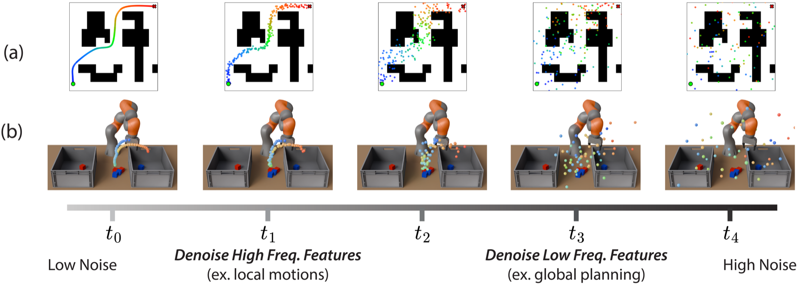
Across five diffusion times the policy first commits to a global path or bin choice at high noise, then refines local motion at low noise, for both a 2D maze and a manipulation task — **Figure 2.** The global-to-local hierarchy, read right-to-left along the backward process. **(a)** a maze policy first commits to a high-level *path* (global planning, high noise $t_4$) then refines it to be collision-free and smooth (local refinement, low noise $t_0$); **(b)** a manipulation policy first picks *which bin*, then refines the grasp. The noise level is a dial between plan and motion.

This is not just a story, it falls straight out of the locality theorem in the next section: at low noise the denoiser's receptive field is short, so the high-level plan (which way through the maze) is fixed early in the backward process and everything after is local refinement. Drag the noise level in the widget below and watch where the smooth target and the jittery demo stop being distinguishable.

◆ the artist's sketch

Denoising a robot action is like an artist who first sketches the overall route through a maze (high noise = the plan) and only later inks the exact wiggle of the line (low noise = the fine motion). Adding noise wipes out the wiggles before it touches the route. So a smooth expert demo and a jittery cheap one, which differ only in the wiggles, become indistinguishable once the noise is high enough.

04Two safe zones, two theorems

The power law does not just suggest the hierarchy, it proves two precise statements (for a clean zero-mean stationary Gaussian model) that pin down exactly where suboptimal data is safe. Each opens one "door" through which $\mathcal{D}_q$ is allowed in.

Theorem 1: fast contraction (the high-noise door)

If the target and suboptimal distributions agree on their low frequencies and differ only in the power-law tail, then adding noise pulls them together fast. A generic result (Daras et al.) already says noise contracts any two bounded distributions, but only as $1/\sigma$ and scaled by their original (possibly near-1) distance. The power law gives a much stronger bound.

$$\text{if } \sigma_t^2 \ge C(f^*)^{-\alpha}:\quad d_{\text{TV}}(p_t,q_t) \le \frac{\sqrt{2}\,C}{\sigma_t^2\sqrt{(2\alpha-1)\,(f^*)^{2\alpha-1}}}, \qquad d_{\text{KL}}(p_t\Vert q_t) \le \frac{4C^2}{(2\alpha-1)\,\sigma_t^4\,(f^*)^{2\alpha-1}}$$

In words: under the power law the noised distributions $p_t,q_t$ contract as $1/\sigma_t^2$ in total variation (and $1/\sigma_t^4$ in KL), and the bound is independent of the original distance. Why so fast? The two distributions disagree only in the high-frequency tail, where the power law puts almost no energy; flat Gaussian noise of variance $\sigma_t^2$ swamps that tiny tail the moment it exceeds it, so the gap closes as $1/\sigma_t^2$ instead of the generic $1/\sigma_t$. So a relatively small $t_\text{min}$ already makes $p_t$ and $q_t$ indistinguishable, and above it the suboptimal data is safe to use because at that noise level it looks exactly like the target.

Theorem 2: locality (the low-noise door)

At low noise the optimal denoiser is a Wiener filter, and the power law forces its kernel to decay as $O(1/m^2)$. The consequence is locality: each output action depends only on a small temporal neighborhood of the input, ignoring everything far away.

$$h^*(x) = \Sigma\,(\Sigma + \sigma_t^2 I)^{-1}\,x, \qquad \big|\,(h^*(x))_i - (h^*(M_i x))_i\,\big| \;\le\; \frac{\alpha\,N\,\lVert x\rVert_\infty}{8L}$$

In words: masking out every input action farther than temporal radius $L$ from index $i$ (that is what $M_i$ does) barely changes that output. The kernel $\Sigma(\Sigma+\sigma_t^2 I)^{-1}$ is a weighted average of nearby inputs whose weights come from the action's own covariance $\Sigma$ damped by the noise $\sigma_t^2$; the power-law $\Sigma$ makes those weights die off as $1/m^2$ with temporal distance $m$, so the bound is governed by the spectral slope $\alpha$ itself and a steeper spectrum makes the denoiser more myopic. At low noise the denoiser never "sees" the global structure of a demonstration, so a sample with wrong global logic but good local motion is safe to learn from for $t\le t_\text{max}$: the wrong plan is outside the receptive field.

◆ the myopic repairman

At low noise the denoiser is a repairman who only looks at a few neighboring stitches to fix the current one and never sees the whole garment. So even if a demonstration's overall pattern is wrong (it sorts blocks into the wrong bin), the local stitching technique it teaches is still good, and the policy can safely copy it. That is locality, and it is why the low-noise door exists.

▮ hold both doors in mind

Before the method, fix the two-door picture in place. High noise → contraction → the $t_\text{min}$ door: the fine differences wash out, so even far-apart distributions look identical and the suboptimal data is safe. Low noise → locality → the $t_\text{max}$ door: the denoiser sees only a short neighborhood, so a globally-wrong demo with good local motion is safe. The harmful middle, where the plan is both sharp and distinguishable, is the only place $\mathcal{D}_q$ must be barred.

05The method: one change to the sampler

Ambient Diffusion Policy is standard Diffusion Policy plus one change to the data sampler. Recall the backbone: noise a clean action chunk, train a denoiser to undo it, then act by reverse diffusion.

$$A_t = A_0 + \sigma_t Z,\ Z\sim\mathcal{N}(0,I);\qquad \mathcal{L}(\theta)=\mathbb{E}\big[\lVert h_\theta(A_t,O,t)-A_0\rVert^2\big];\qquad h^* = \mathbb{E}[A_0\mid A_t,O]$$

In words: add Gaussian noise of growing scale to a chunk of future actions, train a network to predict the clean chunk from the noisy one and the observation. The best possible denoiser is just the conditional mean. This is the object Ambient improves on the target distribution using suboptimal data; everything else (U-Net, 16 actions at 10 Hz, execute 8, 10-step DDIM) is unchanged.

The change is a bouncer on the suboptimal data. High-quality target data $\mathcal{D}_p$ is always admissible. Suboptimal $\mathcal{D}_q$ is admitted only at the two ends, the low-noise door (locality) and the high-noise door (contraction), and barred from the harmful middle band.

$$\mathcal{D}_q \text{ admissible} \iff t\in[0,t_\text{max}]\,\cup\,(t_\text{min},T]; \qquad w_t^{(i)} = \frac{w_i}{\sum_{j\in S_t} w_j}\ \text{ if } i\in S_t,\ \text{else } 0$$

The whole method in one line. Let suboptimal data contribute only where it aligns with the target, never in $(t_\text{max},t_\text{min})$. At OXE scale each dataset $i$ also carries a weight $w_i$ that is renormalized over only the datasets $S_t$ admissible at time $t$. Inference is identical to plain Diffusion Policy: none of this machinery runs at deployment.

How is $t_\text{min}$ found? With a give-up classifier. Train a little detective $c_\phi(A_t,t)$ that, given a noised action chunk, guesses whether it came from the good data or the suboptimal data. Crank up the noise until the detective can no longer tell them apart (its score falls within $\tau$ of $0.5$). That surrender point is $t_\text{min}$.

$$t_\text{min} = \inf\Big\{\, t : \mathbb{E}_{(O,A_0)\sim q,\ A_t\mid A_0}\big[\,c_\phi^*(A_t,t)\,\big] > 0.5 - \tau \,\Big\}$$

In words: operationalize "indistinguishable" by raising noise until a trained classifier gives up. In the 2D maze, with $\tau=0.05$, the classifier surrenders at a noise level of $\sigma_{t_\text{min}}^*\approx0.074$ (the paper reports the cutoff as a noise scale, not a step index). Theorems 3-4 turn this threshold into a guaranteed bound on the LeCam (hence total-variation) distance between $p_t$ and $q_t$, so the cutoff is principled, not heuristic. $t_\text{min}$ can be annotated once per dataset or per individual datapoint; $t_\text{max}$ is set manually here.

The widget below lets you build the sampler. Drag the two gates and watch which demonstrations are let in, then flip to co-training and watch the policy get poisoned.

★ the donut

Because every suboptimal dataset is excluded between its $t_\text{max}$ and its $t_\text{min}$, the intermediate band of noise is sampled only from the clean target $\mathcal{D}_p$. Across the noise axis the suboptimal-data usage has a literal hole in the middle, the "donut" pattern, and that hole is the geometric reason Ambient avoids the harmful regime that co-training sits squarely inside.

Test yourself: why is the middle band the harmful one, and not the ends?

At the ends the suboptimal demo cannot mislead: at low noise the denoiser is local, so it only copies the demo's (good) fine motion and cannot even see its wrong plan; at high noise contraction has blurred the demo onto the same coarse shape as a correct one. Only in the middle is the demo's global plan both fully formed (noise has not blurred it away) and still distinguishable from the target (noise has erased the fine motion that was its only safe contribution). That is precisely the band where a wrong plan gets taught as if it were right, which is why it is the one place to bar $\mathcal{D}_q$.

06Controlled proofs of concept

Four controlled experiments isolate one kind of suboptimality each, with hyperparameters swept per baseline for fairness.

Noisy trajectories. In a 2D maze, $\mathcal{D}_p$ is 50 smooth optimization-based (GCS) trajectories and $\mathcal{D}_q$ is 5000 jittery RRT trajectories that are 5000× cheaper. Both co-training and Ambient reach 99%+ success, but Ambient is about 2× smoother (squared acceleration 31.0 vs co-training's 62.2), and its smoothness-vs-success frontier strictly dominates. On 7-DoF neural motion planning, Ambient leads co-training by about 6 points at $N{=}1$ (65.9% vs 59.9%) and matches it at best-of-100 (91.9% vs 91.3%) while cutting squared acceleration from 32.6 to 20.2.

Sim-to-real. On planar pushing, with 50 target-sim teleop demos and 2000 source-sim planner demos, every Ambient variant beats co-training (84.5%); annotating $t_\text{min}$ per datapoint is best at 93.5%. Locality does not help here, because $\mathcal{D}_p$ and $\mathcal{D}_q$ have genuinely different low-level contact dynamics.

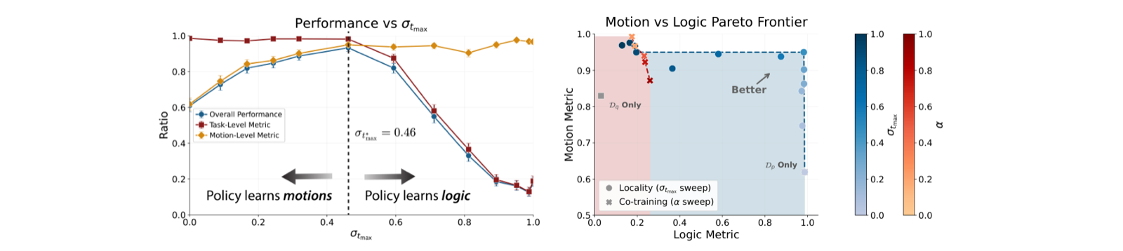
Block-sorting performance vs the locality cutoff: as the cutoff grows the policy first learns local motion, then global logic, with logic plateauing at sigma=0.46 — **Figure 7.** Block sorting (task mismatch), the cleanest demonstration. As the low-noise cutoff $\sigma_{t_\text{max}}$ grows left to right, the policy first acquires good **motion** (the pick-and-place skill, orange) and only later absorbs the **logic** (which bin, dark red), which plateaus right at $\sigma_{t_\text{max}}^*=0.46$. Pushing past that point starts re-teaching the demonstrations' *wrong* logic, so overall performance (blue) falls. The dial is real and tunable.

▮ task mismatch: 98% logic and 95% motion at once

The block-sorting story is the sharpest. Feed the policy 50 correct-sorting demos as $\mathcal{D}_p$ and 200 demos that sort into the opposite bins as $\mathcal{D}_q$. Co-training learns to mis-sort: training on wrong-logic data at all noise levels collapses logic to 26% and success to 22.7%. Ambient restricts that data to low noise, copying its good pick-and-place while never seeing its wrong global plan, and keeps 98.2% logic and 95.0% motion for 93.3% success. A locality-only ablation (suboptimal data at low noise, target at high) reaches 97.9% logic / 93.8% motion, directly confirming the hierarchy.

◆ one demo, traced

Follow a single wrong-bin demonstration through the noise axis. It grasps the block with a clean motion, then places it in the wrong bin. At low noise ($\sigma\le\sigma_{t_\text{max}}^*\!=\!0.46$) only its local pick-and-place sits inside the denoiser's receptive field, so it teaches a good grasp and the wrong bin is invisible: admitted. In the middle band its wrong global plan is both sharp and distinguishable: barred. At very high noise ($\sigma>\sigma_{t_\text{min}}^*$) it has contracted onto the same blur as a correct demo: admitted, and harmless. That one bad demo hands the policy its good grasp and keeps its wrong bin out, which is the whole 98%-vs-26% gap in miniature.

07Scaling to Open X-Embodiment

The controlled experiments use clean, hand-built distribution shifts. The real test is an unstructured mixture: Open X-Embodiment, either OpenVLA's Magic Soup++ (27 datasets, 1,279,774 demos) or a larger Custom OXE (48 datasets, 1,402,606 demos), as the suboptimal pool behind two real-world tasks on a physical robot.

+33%

taller towers than co-training on tower building (15.15 vs 11.35 blocks placed before topple)

+84%

taller towers than data filtering on the same task (15.15 vs 8.20 blocks)

up to 15%

higher table-cleaning success than co-training (about 12% at $\mathcal{D}_p{=}50$, up to 15% per Fig 9)

1.6 vs 2.4

grasp attempts per object vs co-training; and 14.8 s vs 24.9 s time per object

▮ it keeps scaling, and barely needs the weights

Ambient keeps improving as the suboptimal pool grows from Magic Soup++ (1.28M) to Custom OXE (1.40M), while co-training plateaus, evidence that Ambient extracts signal even from the datasets filtering throws away. It is also far more robust to the fragile dataset weights: Ambient drops at most 9% when run unweighted, whereas unweighted co-training was "too dangerous to evaluate on hardware." Because $\mathcal{D}_q$ is only used where $p_t\approx q_t$, the weights stop being load-bearing.

▲ at scale, the high-noise door does most of the work

Honest nuance: the principled classifier method assigns $t_\text{max}=0$ to nearly all OXE datasets, so the paper sets a small $t_\text{max}$ by hand (10 for table cleaning, 5 for tower building). That means at scale the locality (low-noise) door is barely used; almost all the gain comes through the contraction (high-noise) door. "Ambient + Locality" wins on OXE are driven mostly by the $t_\text{min}$ side, not the $t_\text{max}$ side.

08Honest boundaries and the bigger idea

● honest limitations

Ambient only handles distribution shift in the action space, not the observation space (two attempted observation-space fixes did not help, and "suboptimal observations" are ill-defined anyway). The theory is restricted to zero-mean stationary Gaussians, a clean but simplified model. The classifier-based annotation is grounded but does not always beat a costly hyperparameter sweep, and it under-uses locality at scale. The method trains on more data than filtering, so it costs more compute. The user must decide how to split data into $\mathcal{D}_p$ and $\mathcal{D}_q$, a consequential choice the algorithm does not resolve. And gains shrink as $\mathcal{D}_p$ grows: when high-quality data is plentiful, suboptimal data adds less.

The bigger idea is a transferable design principle. Ambient extends Diffusion Policy and imports the Ambient Diffusion / Ambient Diffusion Omni line (used in vision and protein design) into robotics by identifying the spectral power law as the property that makes it apply. It reframes co-training and data filtering as special cases that ignore the noise axis, and it surfaces a learned, data-driven version of the classic hierarchical decomposition (high-level plan plus low-level controller) without any hand-crafted factorization.

The one-sentence takeaway: stop asking which data sources to use and start asking when each should teach. Because robot actions are power-law, diffusion noise cleanly separates the global plan from the local motion, so a single suboptimal demonstration can hand you its good parts and keep its bad parts out, a principle for any diffusion world model trained on mixed-quality data.